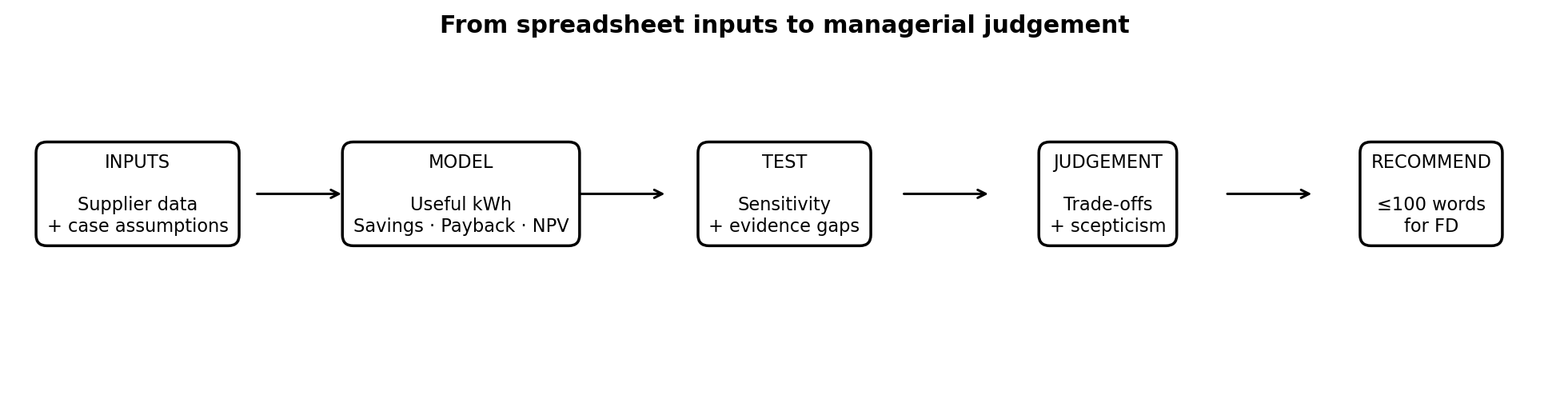
Before we discuss NPV, give me a clean Year-1 comparison.
I want to see what each system produces economically, what it saves after maintenance, and how quickly the capital is recovered. Keep the model traceable to the source data.
Purpose → Outcome → Activity → Evidence
Purpose of this stage: convert supplier and case data into comparable financial measures using an auditable spreadsheet structure.
Outcome for this stage:Construct an auditable spreadsheet model that converts operational solar data into comparable Year-1 financial measures.
You will demonstrate this by: calculating useful generation, gross and net Year-1 savings and simple payback; applying relative and absolute references appropriately; formatting outputs consistently; and creating a decision-relevant visual.
Evidence: completed Your Model!B4:D8, one comparison chart and a one-sentence visual-design rationale.
Excel + Google Sheets · Build
All formulas on this page are identical. Enter them in the same cells and copy them across in the same direction.
Excel formatting Select B5:D6 → Home → Number and choose Currency/Accounting. Select B7:D7 and show two decimal places.
Google Sheets formatting Select B5:D6 → Format → Number → Currency (or use the currency toolbar button). Select B7:D7 → Format → Number → Number and set two decimal places.
Story so far: You understand the inputs and have entered your first formula. Now complete the chain from operating data to payback.
The case · The Financial Director wants comparable numbers
Turn three supplier proposals into one auditable model
Management needs a common basis for comparison. Build the logic in the Your Model sheet: useful generation → gross saving → net saving → simple payback.
Copy B4 across to D4. Relative references should change automatically.
2
Gross Year-1 saving
Gross saving = useful generation × tariff
Select Your Model!B5 and enter:
=B4*'Case Data'!$B$4
Copy across to D5. The first reference changes B4 → C4 → D4; the tariff stays locked at Case Data!$B$4.
NoteFormative feedback · check values
B5 = R231,840; C5 = R287,980; D5 = R321,048.
3
Net Year-1 saving
Net saving = gross saving − maintenance
In Your Model!B6 enter:
=B5-'Case Data'!B17
Copy across to D6. Format B6:D6 as rand currency.
NoteFormative feedback · check values
B6 = R222,840; C6 = R276,980; D6 = R307,048.
4
Simple payback
Simple payback = installed cost ÷ Net Year-1 saving
In Your Model!B7 enter:
='Case Data'!B13/B6
Copy across to D7. Format B7:D7 to two decimal places.
NoteFormative feedback · diagnose your result
Your answers should be approximately A = 2.92, B = 2.96, C = 3.22 years. If not, check percentage formats, cell references, subtraction of maintenance, and numerator/denominator.
Optional Excel skill · rank the paybacks
Use a function rather than ranking by eye
In Your Model!B8 enter:
=RANK.EQ(B7,$B$7:$D$7,1)
Copy across to D8. The final argument 1 means the smallest payback receives rank 1.
NoteFormative feedback · check ranks
System A = 1, System B = 2, System C = 3.
Visual communication task
Create one chart an executive can read in five seconds
Decide which single comparison your chart should communicate.
For a simple-payback chart, use proposal names B3:D3 and payback values B7:D7.
Excel Select B3:D3, then add the non-adjacent B7:D7 range using Ctrl (Windows) or ⌘ (Mac). Choose Insert → Column or Bar Chart → Clustered Column.
Google Sheets The simplest beginner route is to create a small temporary two-row chart source in unused cells (for example H3:J4): copy the three proposal names into row 3 and link row 4 to B7:D7. Select H3:J4 → Insert → Chart → choose Column chart in the Chart editor. This avoids awkward non-adjacent selection.
Give the chart a decision-focused title such as Simple payback by proposal.
Remove anything that does not help a manager compare the three systems.
Write one sentence: “I chose to show ___ because ___.”
Evidence produced: completed Your Model!B4:D8 + one chart + one-sentence design rationale.
Next: management challenges an assumption. Test whether your conclusion survives.